Hue Engine: Reversing the PWM functions
Introduction
This is the third post in the Reversing Philips Hue light driver series.
In the second part, I dumped the PWM data for various brightness / color temperature settings.
Problem statement
There are three functions of two parameters (color temperature, brightness) that define the PWM output channels:
I want to get a mathematical description of the generating function. Ideally exact, but a decently close approximation is fine, too.
The journey
Originally I had no idea where to even begin. I asked ChatGPT for advice as to
how to reverse engineer the two-parameter function. The answer I got was around
sklearn.preprocessing.LinearRegression.
That did not get me anywhere close to fitting the data. I fiddled around
with other python packages, namely scipy.optimize.curve_fit before giving
up, and asking for help on scicomp.
I was pointed at higher-order functions, spline approximation, and symbolic regression.
I tried them all, and mostly failed.
Then I briefly chatted with one of my colleagues (Balazs), who was immensely interested in the point of saturation.
See, the picture above was actually a lie. Actual data looked more like this:
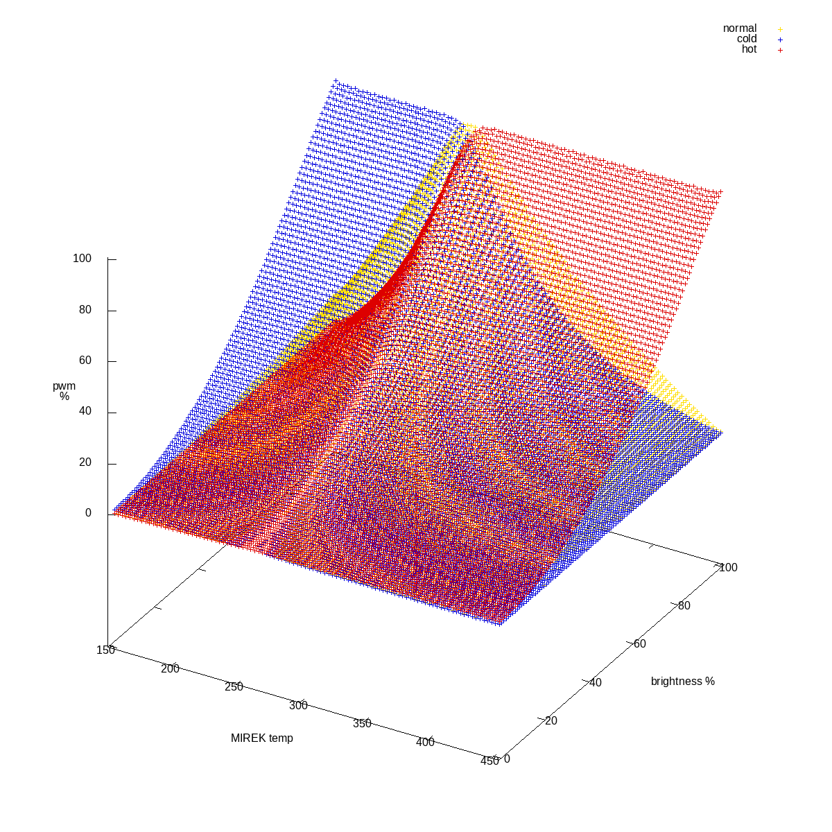 All three channels combined, original sparse data
So I played a bit of a trick on myself by running the data through gnuplot with interpolation.
Balazs mentioned that there’s probably a sharp transition around the saturation, and that I should explore that further. Plus, that “everything around light is logarithmic”.
I decided to dense up the data, that’s the reason for the weird combos in
pwm-dumper.rb:
combos = []

mireks = (153.step(454, 5) + [454]).to_a
brightnesses = 0.step(100, 5).to_a

# Basic cartesian for 5-point matrix
combos += mireks.product(brightnesses)

# points around saturation
combos += (245..268).to_a.product(brightnesses)

# lower brightness
combos += mireks.product((0..15).to_a)

# every mirek at 90,95,100 brightness
combos += (153..454).to_a.product([90, 95, 100])

# every mirek at 90..100 brightness (step 2)
combos += (153..454).to_a.product(90.step(100, 2).to_a)

# DRY
combos.sort!.uniq!
Because I wanted to collect more data.
With that the shape is somewhat different:
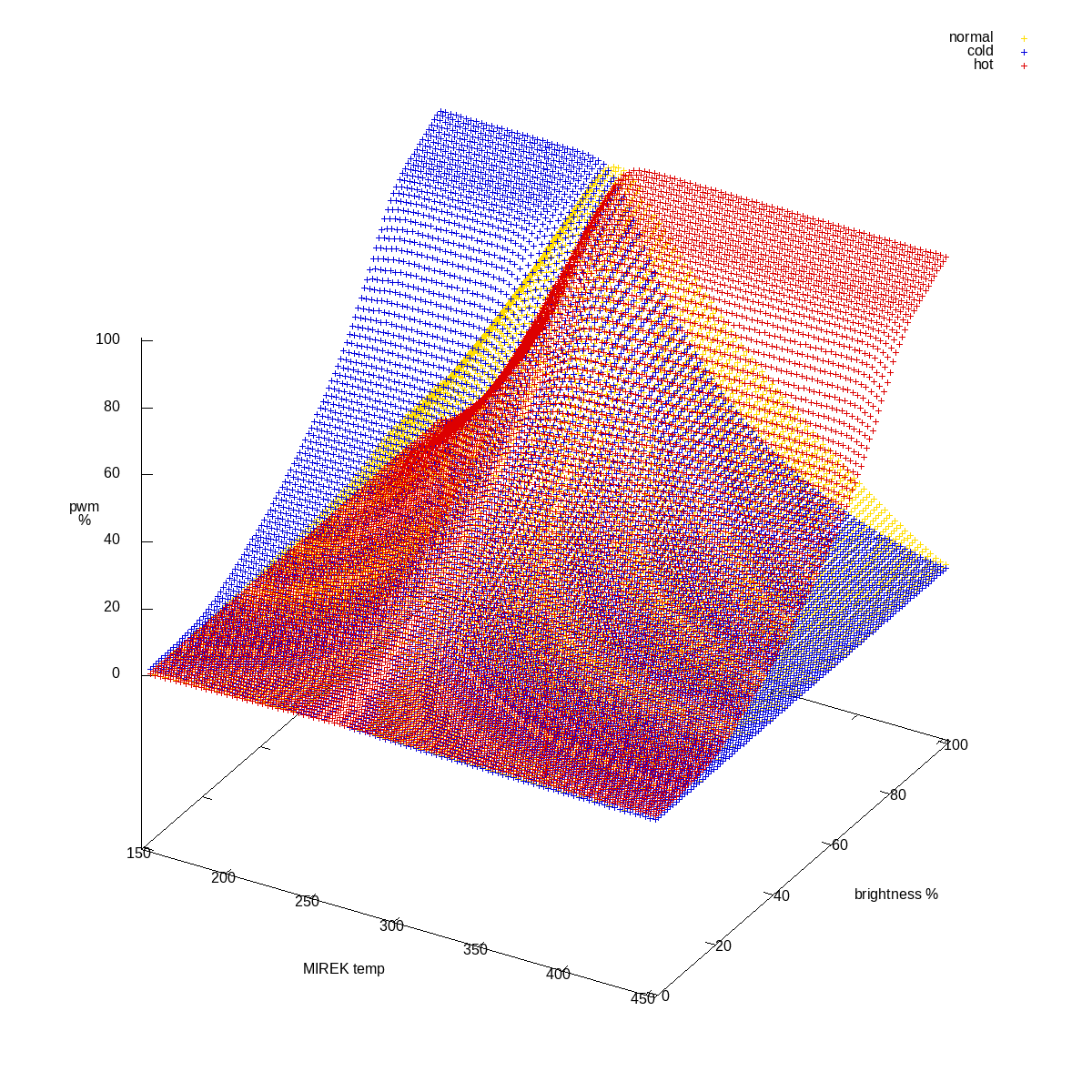 All three channels combined, final data
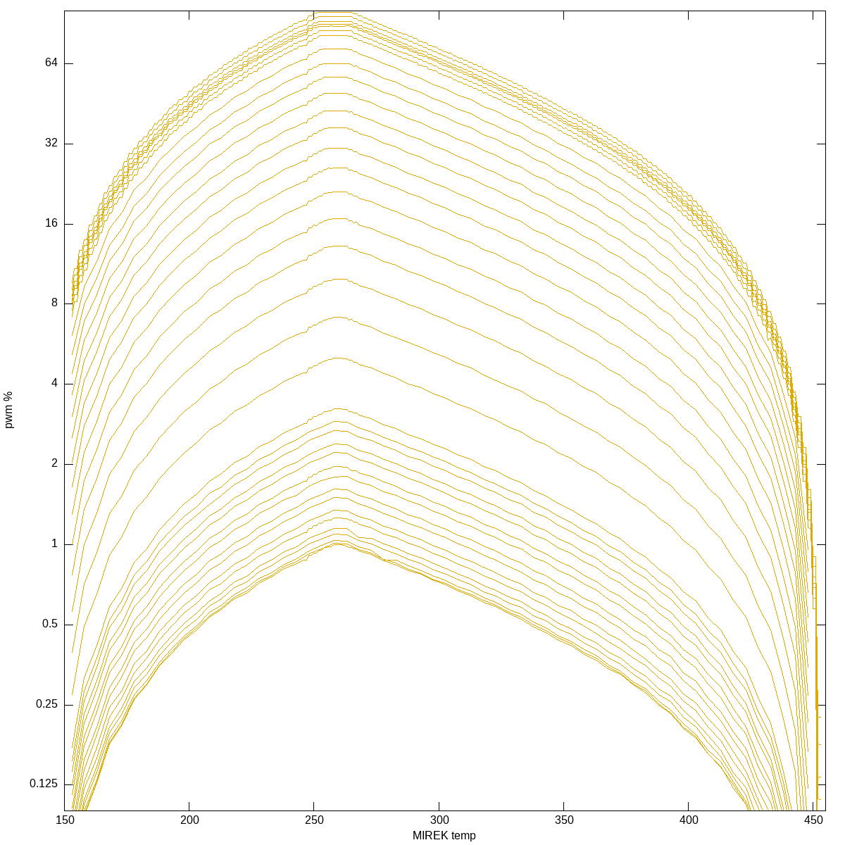
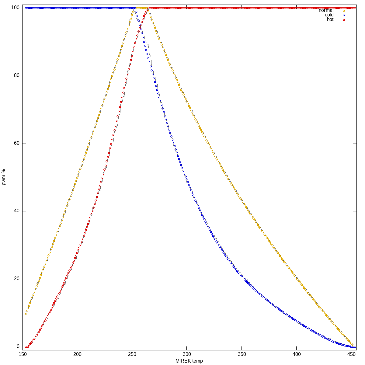
In order to get somewhere, I decided to project to 2d, to better see the curves:
Which was strangely symmetrical1. That got me thinking that I could maybe approximate brightness separately from the color-temperature.
So I took brightness at specific color temperature points (258 for normal,
223 for cold, 303 for hot), dumped it to json, and tried running linear
regression on that:
#!/usr/bin/env python3

import numpy as np
from scipy.optimize import curve_fit
from sklearn.preprocessing import PolynomialFeatures
from sklearn.linear_model import LinearRegression
from sklearn.metrics import mean_squared_error
import json

with open('pwm-table-brightness.json', 'r') as file:
    data = json.load(file)

brightness = np.array(data["brightness"])
normal = np.array(data["normal"])
cold = np.array(data["cold"])
hot = np.array(data["hot"])

def f(X, a, b, c):
    x = X
    return (a + b*x + c*x**2)

out = dict()

def pretty_print(name, popt, pcov, x_data, y_data):
    print(name + ":")
    print('popt:', popt)
    print('pcov:', pcov)
    perr = np.sqrt(np.diag(pcov))
    print('perr:', perr)
    y_pred = f((x_data), *popt)
    mse = np.mean((y_data - y_pred)**2)
    print("mse:", mse)
    print()

popt, pcov = curve_fit(f, (brightness), normal)
out['normal'] = list(popt)
pretty_print('normal', popt, pcov, (brightness), normal)

popt, pcov = curve_fit(f, (brightness), cold)
out['cold'] = list(popt)
pretty_print('cold', popt, pcov, (brightness), cold)

popt, pcov = curve_fit(f, (brightness), hot)
out['hot'] = list(popt)
pretty_print('hot', popt, pcov, (brightness), hot)

with open('brightness-curves.json', 'w') as out_file:
    json.dump(out, out_file, indent=4)
And it worked!
$ ./fit-brightness.py
normal:
popt: [ 9.99462593e-01 -3.40382133e-04  9.90325710e-03]
pcov: [[ 1.03065521e-05 -4.85098868e-07  4.14057014e-09]
 [-4.85098868e-07  3.92993010e-08 -3.84299001e-10]
 [ 4.14057014e-09 -3.84299001e-10  3.96309146e-12]]
perr: [3.21038193e-03 1.98240513e-04 1.99075148e-06]
mse: 8.65420496797531e-05

cold:
popt: [ 1.00003168e+00 -6.77564568e-05  9.90060890e-03]
pcov: [[ 8.83310608e-06 -4.15743520e-07  3.54855845e-09]
 [-4.15743520e-07  3.36806564e-08 -3.29354462e-10]
 [ 3.54855845e-09 -3.29354462e-10  3.39646949e-12]]
perr: [2.97205419e-03 1.83522904e-04 1.84295130e-06]
mse: 7.4171072704184e-05

hot:
popt: [9.98913762e-01 3.69293940e-05 9.89944166e-03]
pcov: [[ 8.09243226e-06 -3.80831025e-07  3.25035489e-09]
 [-3.80831025e-07  3.08507557e-08 -3.01674354e-10]
 [ 3.25035489e-09 -3.01674354e-10  3.11100027e-12]]
perr: [2.84472007e-03 1.75643832e-04 1.76380279e-06]
mse: 6.795975687969396e-05
Graphing that was a thing of beauty2:
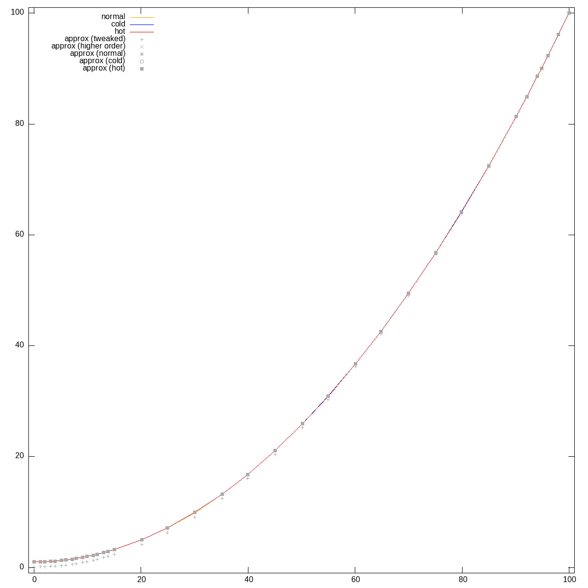 brightness approximation vs gathered data
For all three channels the curve is virtually the same.
Half of the problem is solved!
I also retried the PySR (symbolic regression) on the brightness alone, and the solutions it came up with were interesting:
#PySR attempts at figuring out the brightness:
x0, x1 = mirek, brightness

# Try 1:
(Math.exp(Math.sin(Math.log(x0 ** -4.2384))) + -0.2912) *
 ((0.0038482 * (x1 * x1)) + 0.40689)

# Try 2:
((x1 * 0.003885924) *
 (x1 * (Math.exp(Math.sin(Math.log(x0 ** -4.238486))) + -0.28776997))) +
Math.sin(x0 ** 0.58981854)

# Three:
((Math.sin(((2392.413 / x0) - 2.2254682) / 1.5551411) + -1.1892307) *
 ((x1 / -2.2668383) - -5.230437)) +
(x0 ** -0.32174507)

# Four:
((Math.cos(x0 / ((x0 + 8.137459) ** 0.548065)) - -1.2045676) *
 (x1 * (x1 - -10.18817))) /
(x0 + -1.2525864)
Neither of them fits any better, btw. It’s hard to beat the parabola.
Figuring out the color-temperature curves
For the second half, I basically dumped the curves corresponding to 100% brightness to a json (again).
But this time I only chose the non-saturating parts – heeding Balazs’ advice about cutting off saturation.
Plus, I cut the normal curve in half – each slope separately.
The fit-pwmcurve.py script is almost the same, only uses higher
order polynomial:
#!/usr/bin/env python3

import numpy as np
from scipy.optimize import curve_fit
from sklearn.preprocessing import PolynomialFeatures
from sklearn.linear_model import LinearRegression
from sklearn.metrics import mean_squared_error
import json

with open('pwm-table-fullbright.json', 'r') as file:
    data = json.load(file)

mirek_n1 = np.array(data["mirek_n1"])
mirek_n2 = np.array(data["mirek_n2"])
mirek_c = np.array(data["mirek_c"])
mirek_h = np.array(data["mirek_h"])
normal1 = np.array(data["normal1"])
normal2 = np.array(data["normal2"])
cold = np.array(data["cold"])
hot = np.array(data["hot"])

def f(X, a, b, c, d, e, f):
#def f(X, a, b, c):
    x = X
    #return (a + b*x + c*x**2)
    return (a + b*x + c*x**2 + d*x**3 + e*x**4 + f*x**5)

out = dict()

def pretty_print(name, popt, pcov, x_data, y_data):
    print(name + ":")
    print('popt:', popt)
    print('pcov:', pcov)
    perr = np.sqrt(np.diag(pcov))
    print('perr:', perr)
    y_pred = f((x_data), *popt)
    mse = np.mean((y_data - y_pred)**2)
    print("mse:", mse)
    print()

popt, pcov = curve_fit(f, (mirek_n1), normal1)
out['normal1'] = list(popt)
pretty_print("normal1", popt, pcov, (mirek_n1), normal1)

popt, pcov = curve_fit(f, (mirek_n2), normal2)
out['normal2'] = list(popt)
pretty_print("normal2", popt, pcov, (mirek_n2), normal2)

popt, pcov = curve_fit(f, (mirek_c), cold)
out['cold'] = list(popt)
pretty_print("cold", popt, pcov, (mirek_c), cold)

popt, pcov = curve_fit(f, (mirek_h), hot)
out['hot'] = list(popt)
pretty_print("hot", popt, pcov, (mirek_h), hot)

with open('pwm-curves.json', 'w') as out_file:
    json.dump(out, out_file, indent=4)
And again, more or less success!
$ ./fit-pwmcurve.py
normal1:
popt: [-6.64576279e+02  1.54463883e+01 -1.53120763e-01  7.87165097e-04
 -1.99199066e-06  1.99958433e-09]
pcov: [[ 2.08112820e+06 -5.26665821e+04  5.29355676e+02 -2.64169984e+00
   6.54631067e-03 -6.44532249e-06]
 [-5.26665821e+04  1.33370507e+03 -1.34140119e+01  6.69849733e-02
  -1.66099443e-04  1.63639238e-07]
 [ 5.29355676e+02 -1.34140119e+01  1.35002861e-01 -6.74596769e-04
   1.67383733e-06 -1.65008005e-09]
 [-2.64169984e+00  6.69849733e-02 -6.74596769e-04  3.37307620e-06
  -8.37475624e-09  8.26106428e-12]
 [ 6.54631067e-03 -1.66099443e-04  1.67383733e-06 -8.37475624e-09
   2.08061843e-11 -2.05364940e-14]
 [-6.44532249e-06  1.63639238e-07 -1.65008005e-09  8.26106428e-12
  -2.05364940e-14  2.02827454e-17]]
perr: [1.44261159e+03 3.65199270e+01 3.67427354e-01 1.83659364e-03
 4.56137965e-06 4.50363691e-09]
mse: 0.27130540598011904

normal2:
popt: [ 2.82060879e+02  1.97594522e+00 -2.75937315e-02  1.04037626e-04
 -1.70830613e-07  1.05251876e-10]
pcov: [[ 2.85378756e+04 -4.07703744e+02  2.31089911e+00 -6.49665780e-03
   9.06029906e-06 -5.01553042e-09]
 [-4.07703744e+02  5.82909617e+00 -3.30649902e-02  9.30258061e-05
  -1.29830043e-07  7.19217666e-11]
 [ 2.31089911e+00 -3.30649902e-02  1.87700343e-04 -5.28476718e-07
   7.38104026e-10 -4.09180744e-13]
 [-6.49665780e-03  9.30258061e-05 -5.28476718e-07  1.48905170e-09
  -2.08122909e-12  1.15459425e-15]
 [ 9.06029906e-06 -1.29830043e-07  7.38104026e-10 -2.08122909e-12
   2.91101687e-15 -1.61608217e-18]
 [-5.01553042e-09  7.19217666e-11 -4.09180744e-13  1.15459425e-15
  -1.61608217e-18  8.97814975e-22]]
perr: [1.68931571e+02 2.41435212e+00 1.37003775e-02 3.85882326e-05
 5.39538402e-08 2.99635608e-11]
mse: 0.006974028051178422

cold:
popt: [-2.70308303e+03  4.98116995e+01 -3.23154212e-01  9.85997632e-04
 -1.45136896e-06  8.34172592e-10]
pcov: [[ 5.06924244e+05 -7.39439590e+03  4.27063357e+01 -1.22095400e-01
   1.72835522e-04 -9.69432519e-08]
 [-7.39439590e+03  1.07964881e+02 -6.24148855e-01  1.78609082e-03
  -2.53066689e-06  1.42070670e-09]
 [ 4.27063357e+01 -6.24148855e-01  3.61166666e-03 -1.03450103e-05
   1.46710519e-08 -8.24362266e-12]
 [-1.22095400e-01  1.78609082e-03 -1.03450103e-05  2.96590996e-08
  -4.21002537e-11  2.36770736e-14]
 [ 1.72835522e-04 -2.53066689e-06  1.46710519e-08 -4.21002537e-11
   5.98139094e-14 -3.36688140e-17]
 [-9.69432519e-08  1.42070670e-09 -8.24362266e-12  2.36770736e-14
  -3.36688140e-17  1.89683205e-20]]
perr: [7.11986126e+02 1.03906151e+01 6.00971436e-02 1.72218174e-04
 2.44568823e-07 1.37725526e-10]
mse: 0.4012776209257108

hot:
popt: [ 8.79835997e+03 -2.26331852e+02  2.30636305e+00 -1.16593419e-02
  2.92757451e-05 -2.91413229e-08]
pcov: [[ 1.09785188e+06 -2.70992296e+04  2.65148674e+02 -1.28561968e+00
   3.08967716e-03 -2.94502444e-06]
 [-2.70992296e+04  6.69484813e+02 -6.55602586e+00  3.18145015e-02
  -7.65206663e-05  7.29957072e-08]
 [ 2.65148674e+02 -6.55602586e+00  6.42549032e-02 -3.12069847e-04
   7.51206580e-07 -7.17171085e-10]
 [-1.28561968e+00  3.18145015e-02 -3.12069847e-04  1.51689381e-06
  -3.65438912e-09  3.49158219e-12]
 [ 3.08967716e-03 -7.65206663e-05  7.51206580e-07 -3.65438912e-09
   8.81093356e-12 -8.42500606e-15]
 [-2.94502444e-06  7.29957072e-08 -7.17171085e-10  3.49158219e-12
  -8.42500606e-15  8.06220472e-18]]
perr: [1.04778427e+03 2.58744046e+01 2.53485509e-01 1.23162243e-03
 2.96832167e-06 2.83940218e-09]
mse: 0.26053485003543214
There was a slight issue with the cold channel (and to a lesser
degree with the hot channel), which I worked around by injecting
fake data:
# Manual curve tuning using fake data (sigh)
data_fullbright['mirek_c'] << 450
data_fullbright['cold'] << 0.5
data_fullbright['mirek_c'] << 452
data_fullbright['cold'] << 0.5
data_fullbright['mirek_c'] << 454
data_fullbright['cold'] << 0.2
data_fullbright['mirek_c'] << 456
data_fullbright['cold'] << -0.3
data_fullbright['mirek_c'] << 458
data_fullbright['cold'] << -0.8

data_fullbright['mirek_h'] << 152
data_fullbright['hot'] << -1
But other than that, pretty nice fit:
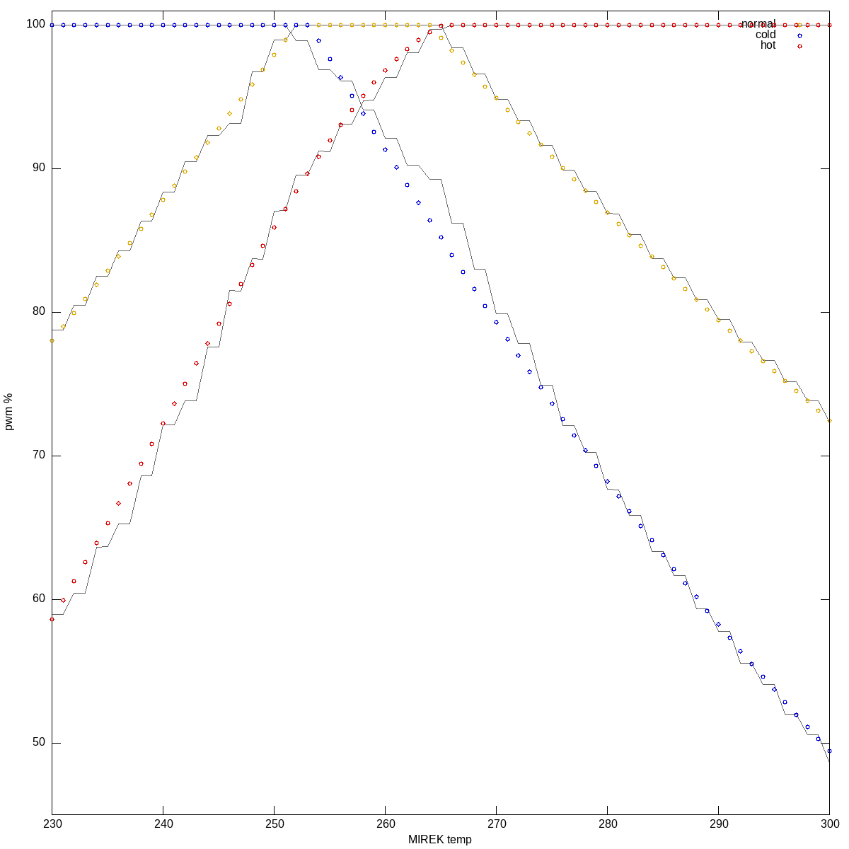 color temp curves, restricted to 230..300
Putting it together
To put it together, I basically wrapped the two JSON output files in Ruby, and for the color temperature curve I stitched the individual parts together for the various intervals.
It ain’t pretty, but it works:
#!/usr/bin/env ruby

require 'json'
require 'pp'

# Correct brightness, optionally using one of the alt curve approximations
def correct_brightness(brightness, name = 'normal')
  # ./fit-brightness.py -- for now.
  $brightnesses ||= JSON.parse(File.read('brightness-curves.json'))
  a, b, c = $brightnesses[name]
  x = brightness
  (a + b*x + c*x**2)
end

def _pwm_for(name, mirek)
  # ./fit-pwmcurve.py -- for now.
  $pwm_curves ||= JSON.parse(File.read('pwm-curves.json'))
  curve = $pwm_curves[name]

  x = mirek
  a, b, c, d, e, f = *curve
  out = (a + b*x + c*x**2 + d*x**3 + e*x**4 + f*x**5)

  # clamp
  if out > 100.0
    100.0
  elsif out < 0.0
    0.0
  else
    out
  end
end

# Approximate PWM value for channel name given mirek and brightness
def pwm_approximate(name, mirek, brightness)
  pwm100 = if name == 'normal'
	     case mirek
	     when 153..252
	       _pwm_for('normal1', mirek)
	     when 265..454
	       _pwm_for('normal2', mirek)
	     else
	       100.0
	     end
	   elsif name == 'cold'
	     if mirek > 449
	       0.0
	     elsif (251..454).include?(mirek)
	       _pwm_for('cold', mirek)
	     else
	       100.0
	     end
	   elsif name == 'hot'
	     if mirek < 156
	       0.0
	     elsif (153..266).include?(mirek)
	       _pwm_for('hot', mirek)
	     else
	       100.0
	     end
	   else
	     0.0
	   end

  (pwm100 * correct_brightness(brightness, name)/100.0)
end
I was obviously curious how well it stacks up. I evaluated the entire
space and drew delta of actual - approximated3:
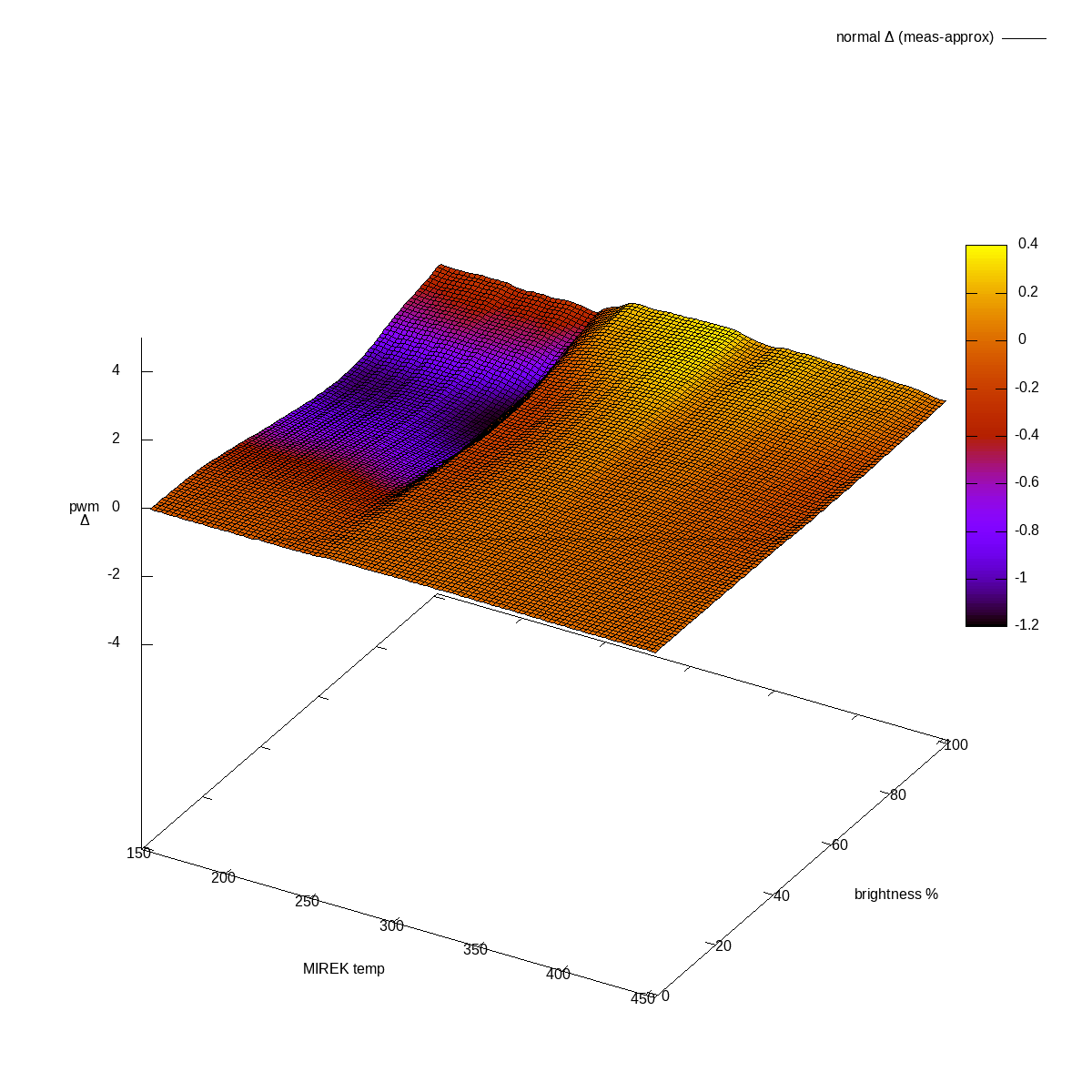 Normal channel, difference actual-approximated
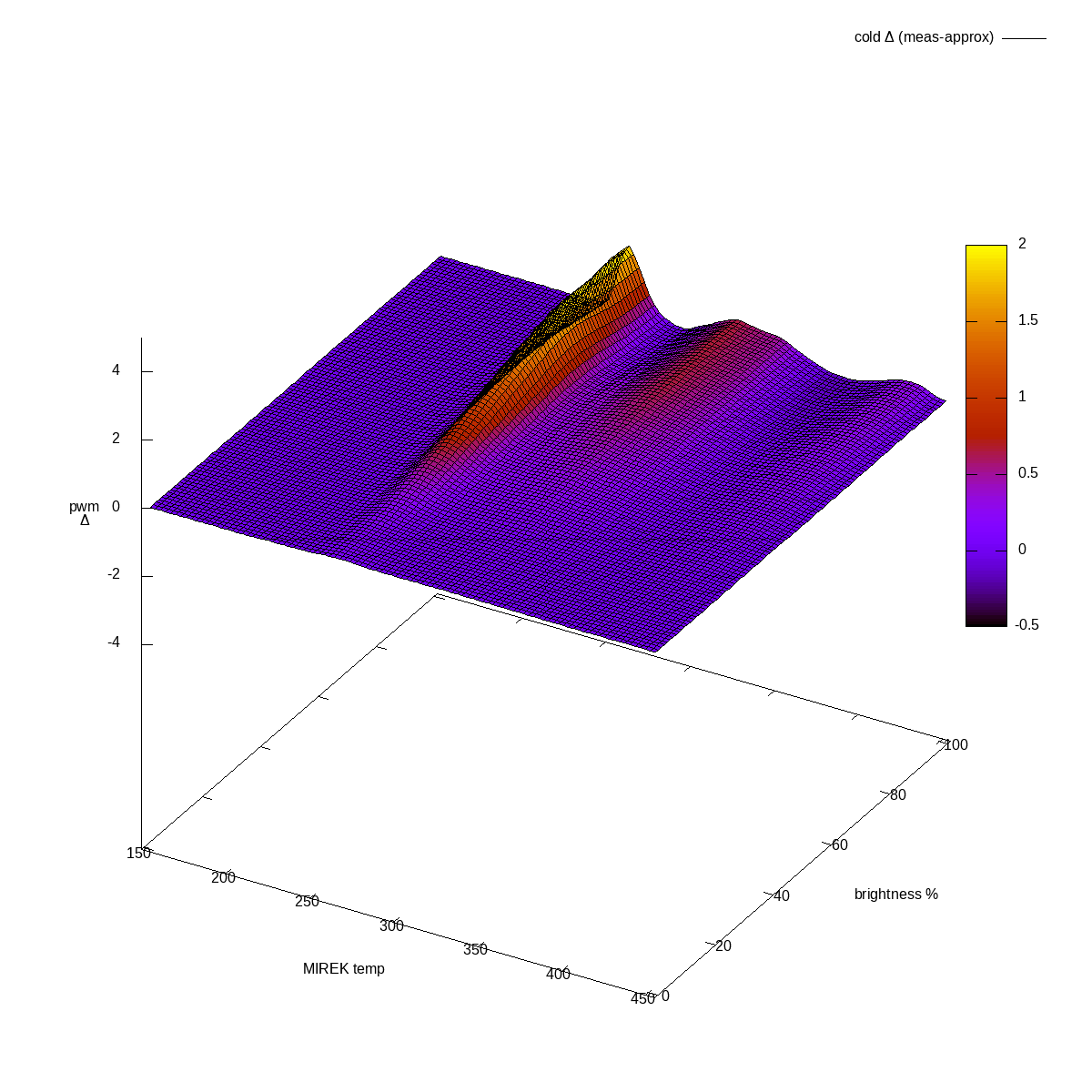 Cold channel, difference actual-approximated
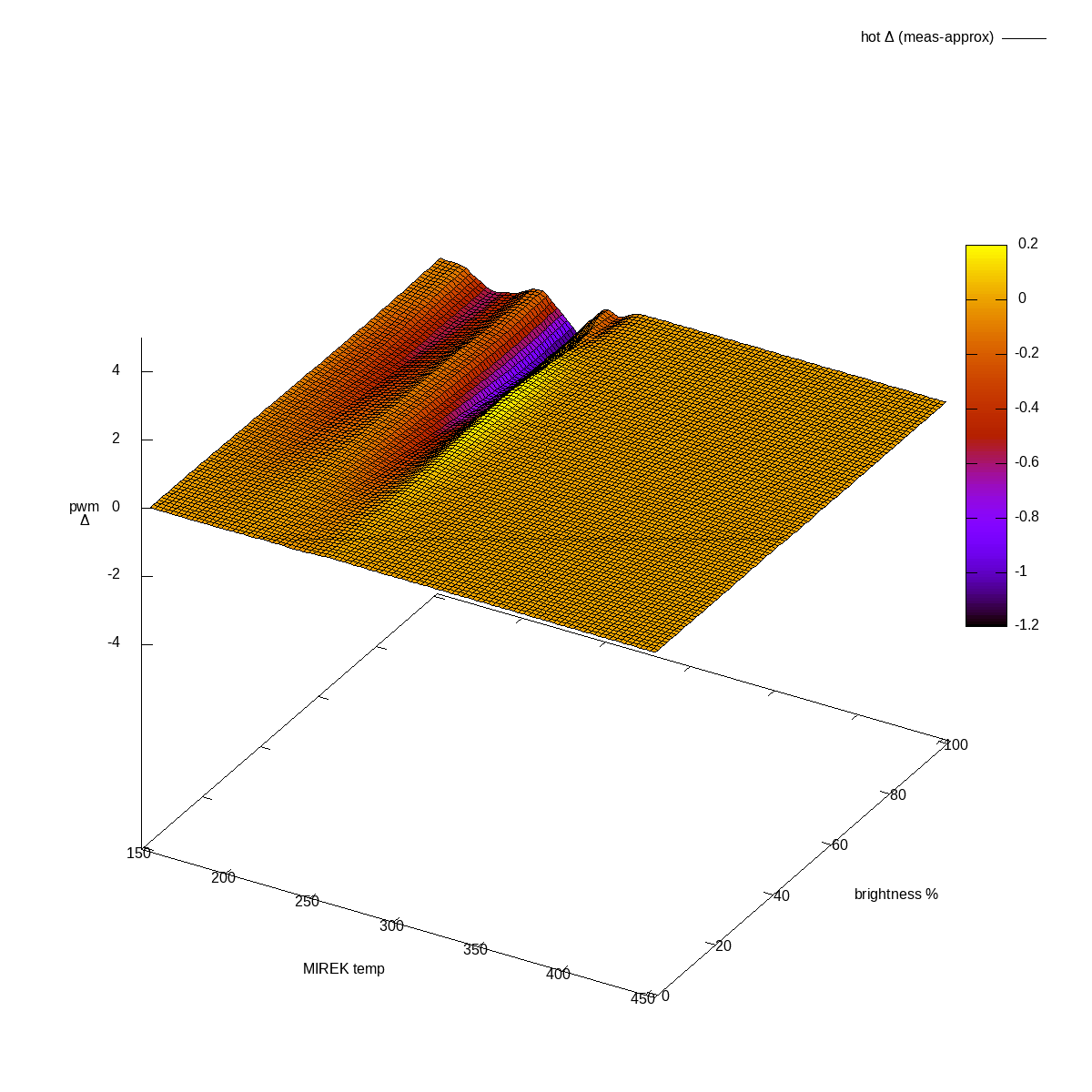 Hot channel, difference actual-approximated
Plus the same in percents (diff divided by actual value):
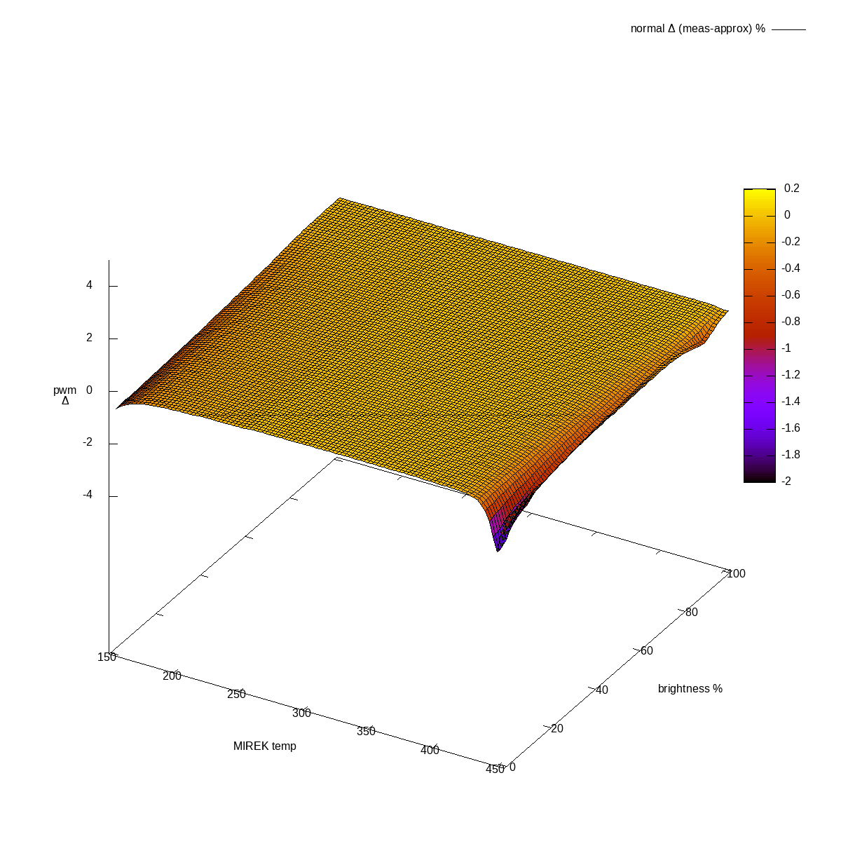 Normal channel, difference actual-approximated, in %
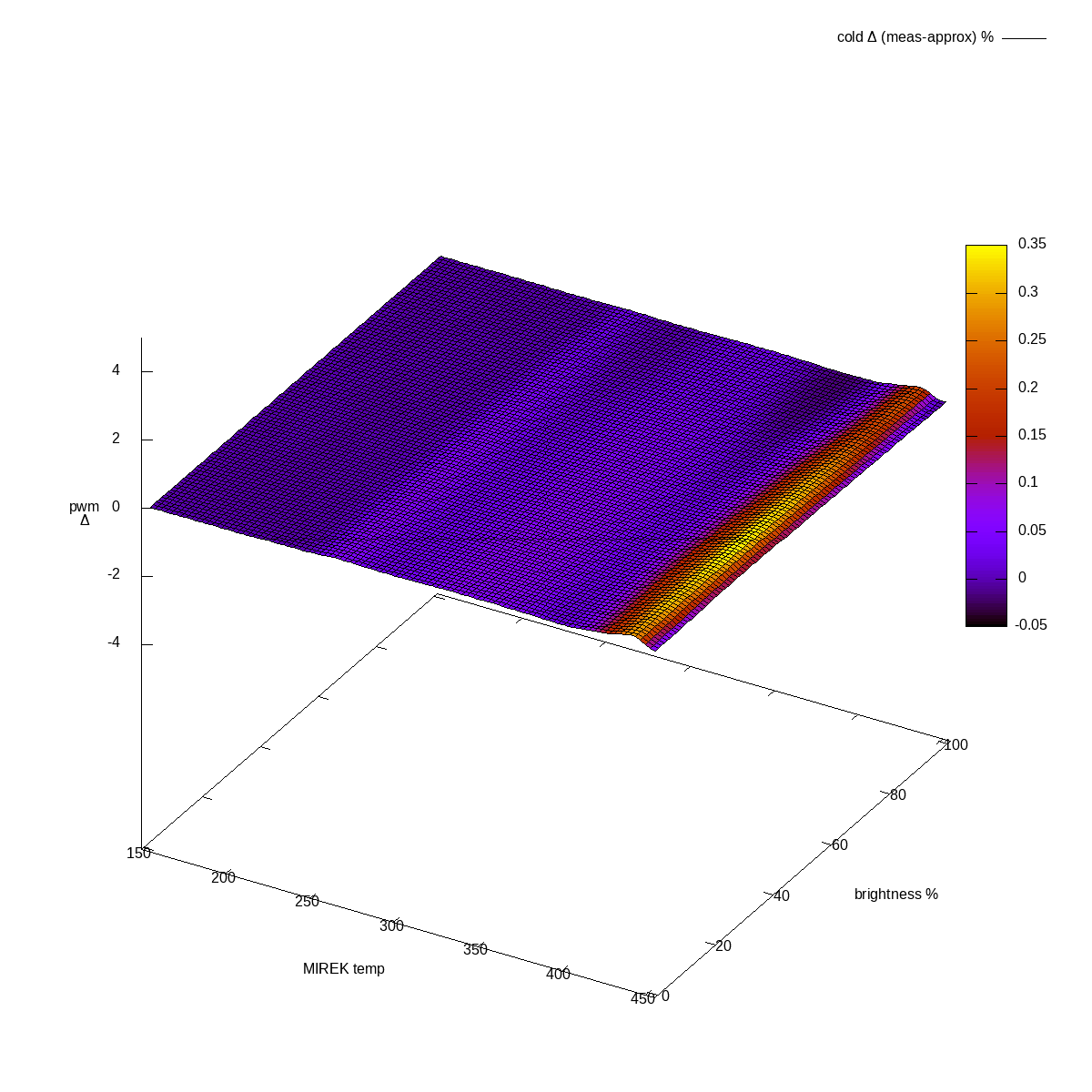 Cold channel, difference actual-approximated, in %
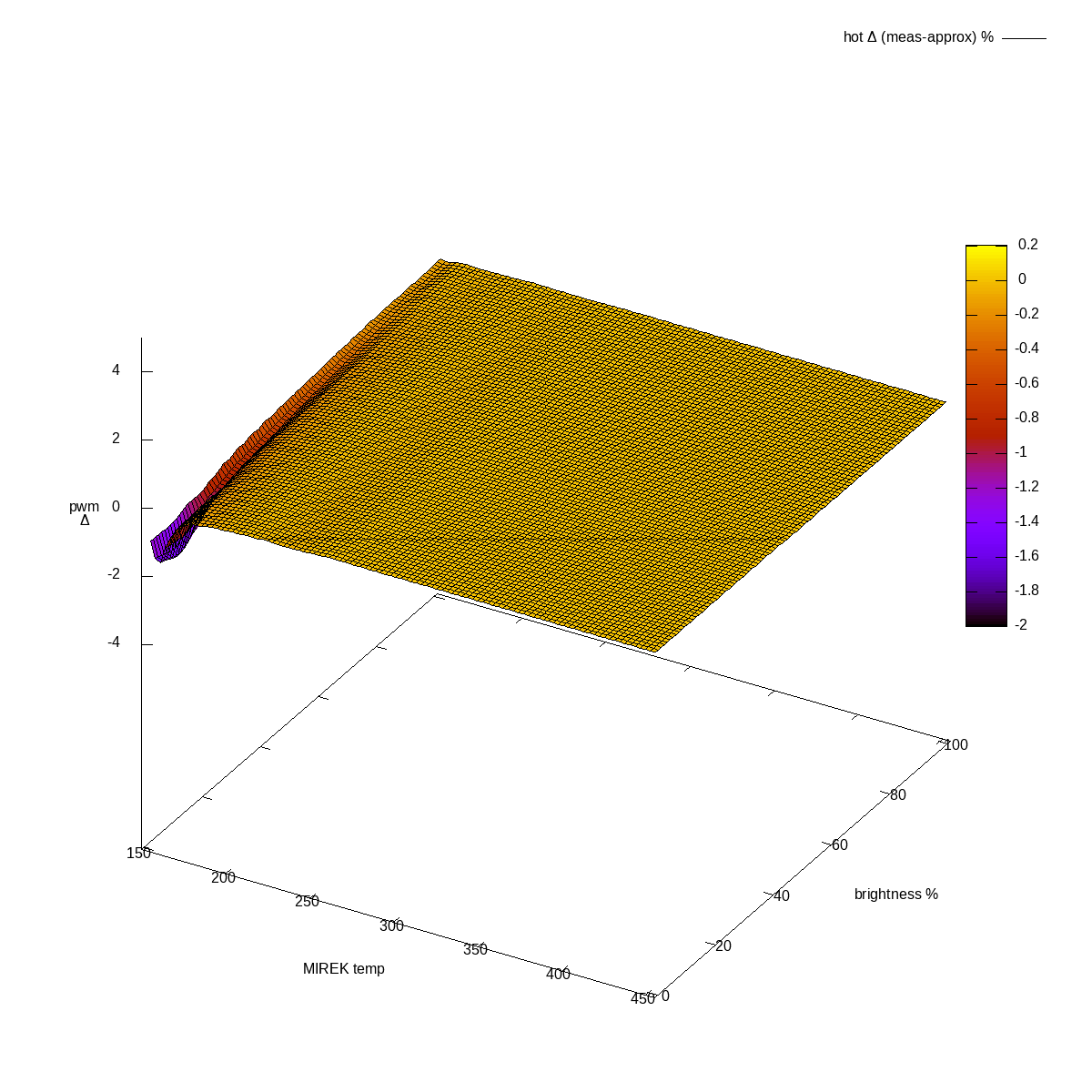 Hot channel, difference actual-approximated, in %
Closing words
Unless I messed up in some major way4, I now have the math description needed for driving the light.
Question remains whether I can efficiently calculate the
a + b*x + c*x**2 + d*x**3 + e*x**4 + f*x**5 on ESP32-C6.
If not, I can always revert to using tables.
In any case, breadboarding some prototype is going to be my next step.
Stay tuned.
-
Pay no attention to the
tweakedfunc, that was me manually trying to simplify to[0.1 -3.4e-04 10e-03]. Mostly works, but undershoots at lower brightness. ↩ -
Originally I just drew one plot over the other, but the difference was imperceptible. ↩
-
In the unlikely event that you want to check my homework (or simply want some of the code I wrote for this), ask. ↩
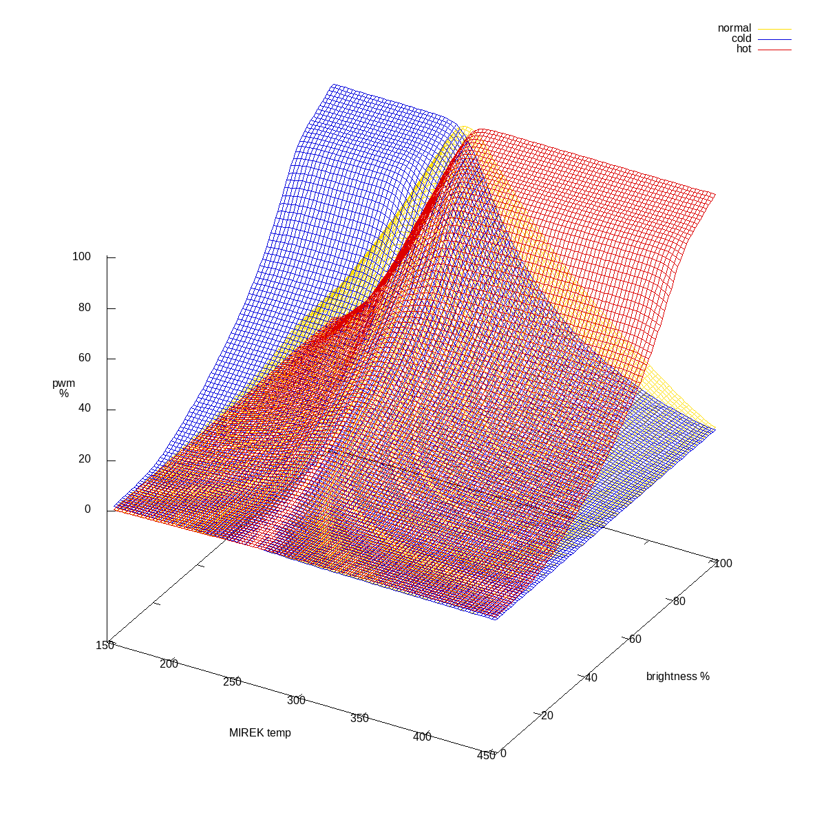 All three channels combined
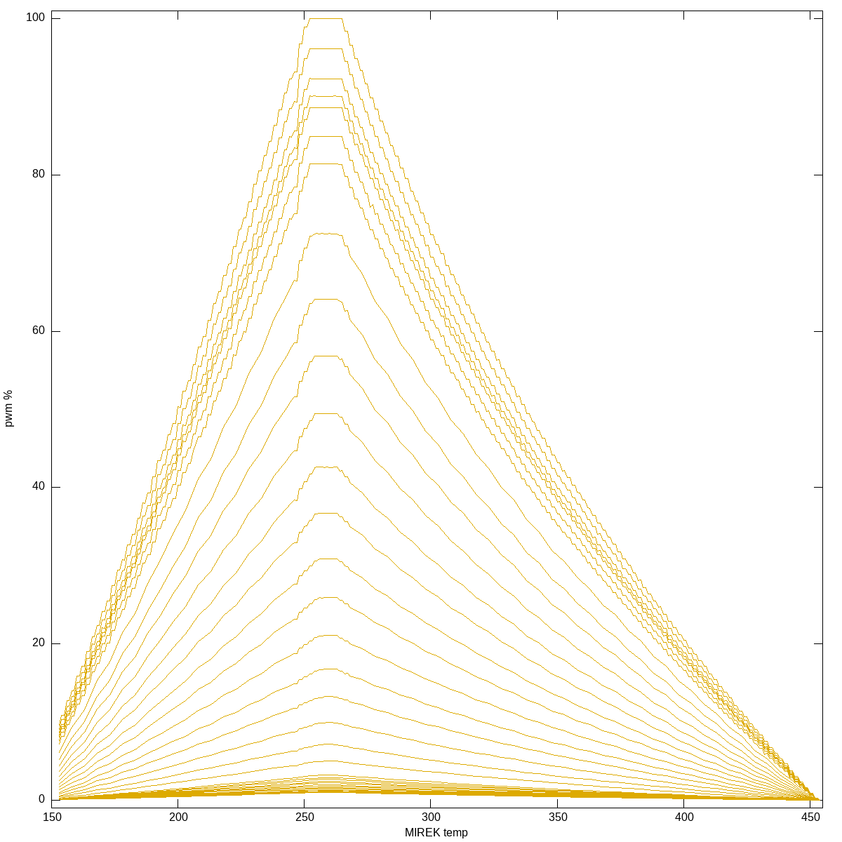 Normal channel, 2d plot
 Normal channel, 2d log-plot
 color temp curves, full