Failing to calibrate flame-s-vis-nir-es spectrometer

Problem statement

Ever since I bought me the Torch Bearer Y21 spectrometer and borrowed another cheap-o spectrometer (Hopoocolor HPCS-320D, 370-780nm) from a friend, I’ve been suffering from Segal’s law:

A man with a watch knows what time it is. A man with two watches is never sure.

The obvious non-solution is to throw a third device in the mix¹. Right?

Unfortunately unbeknownst to me, fancy (precise) spectrometers, like Ocean Optics Flame-S-VIS-NIR-ES², don’t come “calibrated in absolute radiometric units”.

Worse yet, not being “calibrated in absolute radiometric units” means something different than I naïvely expected.

Expectation:

The readout is linear across the entire wavelength range, just the correspondence between Y axis and absolute value isn’t clear

Reality:

The readout across the wavelength range is highly non-linear

The only way to get the spectrometer to display proper sun spectrum instead of the following “garble”³ is to calibrate it.

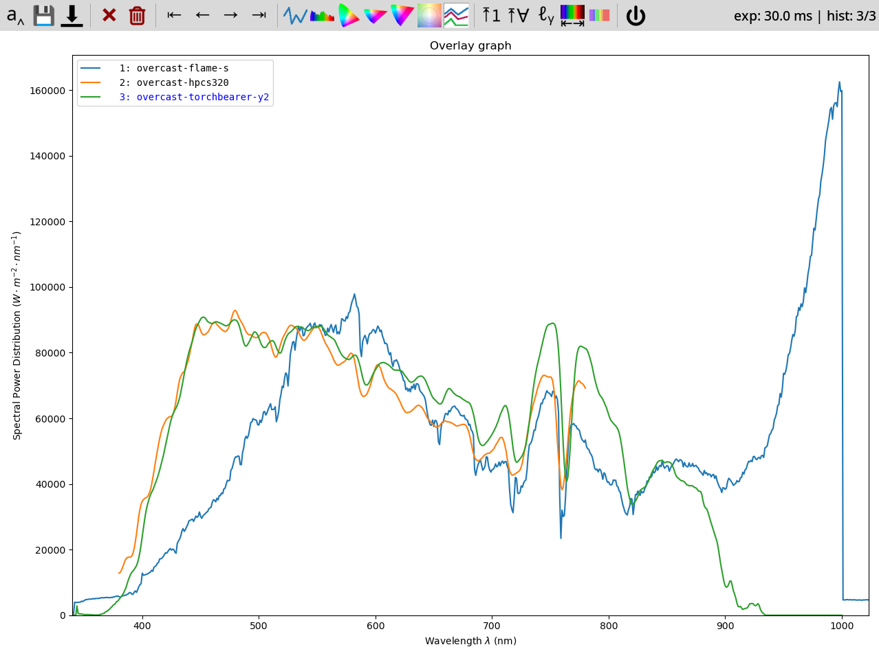
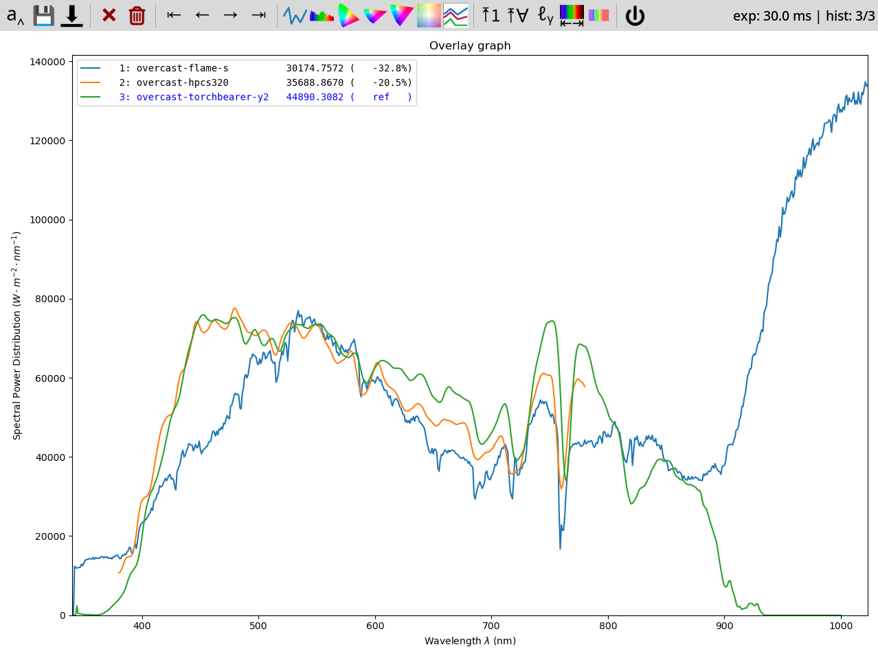
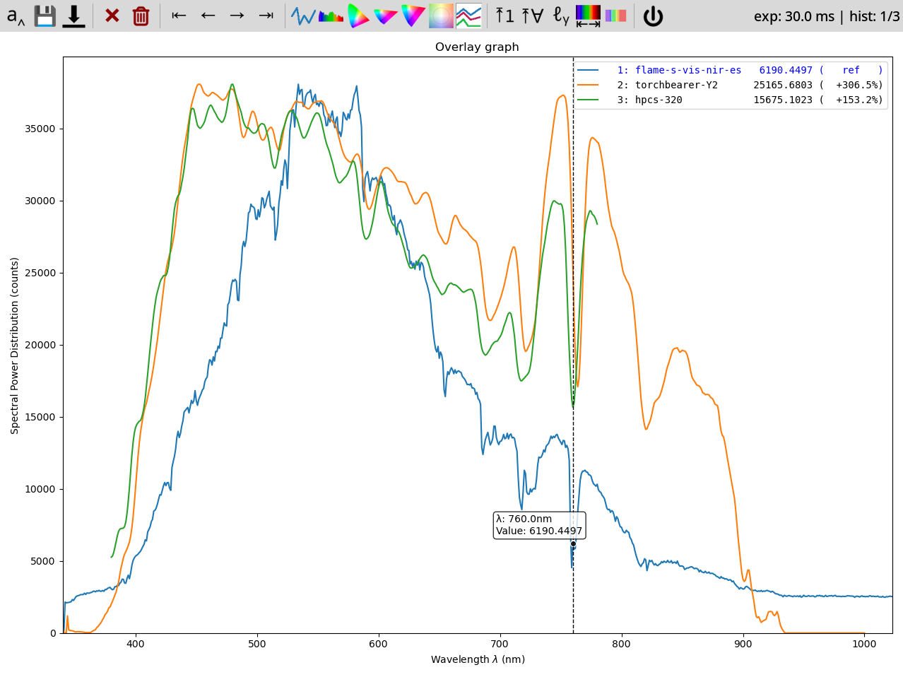comparison of the same spectra across two cheapo chinese (green, orange) and a fancy one (blue)

How not to do that⁴?

Read on… :-)

Root cause of the problem

Freaking out that I bought a lemon, I briefly chatted with Jürgen Söchtig from gmp.ch who calmed me down and explained that what I’m seeing is intrinsic to high-end devices, because they’re mainly used for relative measurements.

Before he could answer a few follow-up questions, I managed to figure out why I’m seeing what I’m seeing.

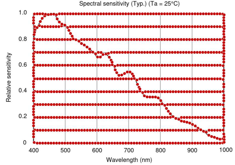
The issue is with the image sensor. The Flame-S has either Sony ILX511 or Sony ILX511B sensor with 2048 B&W pixels.

And one crucial design feature (“flaw”):

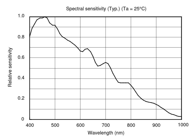Spectral sensitivity of SONY ILX511 (from datasheet)

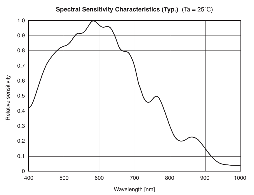Spectral sensitivity of SONY ILX511B (from datasheet)

They are nowhere near linear across the wavelength range⁵.

And the sensor isn’t even the only thing in the optical pathway:

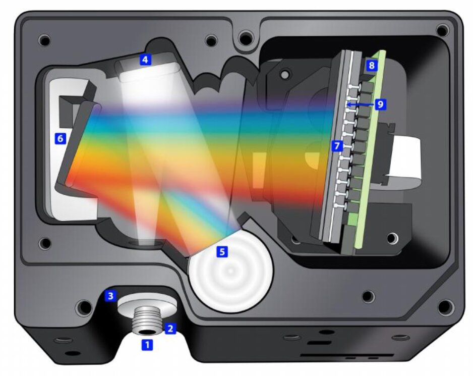Ocean Optics Flame Spectrometer from the inside (labels in the manual above)

So there’s bound to be more fun to be had⁶.

First attempt at solving this

Well, if the datasheet says “this is the curve of the sensor”, translating the curve to floats and adjusting spectra I read out was my first attempt.

The lesson learned: how does one translate the curve in the age of “AI”.

I discovered WebPlotDigitizer which is an awesome tool. You tell it which pixels are which X coords, which are which Y coords, and with a bit of convincing it spits out CSV.

Sounds easy enough.

Spec sheet in hand, I uploaded the PDF, marked all that was necessary, and then discovered that since the datasheet is monochrome, WebPlotDigitizer takes the grid as points too. Ouch.

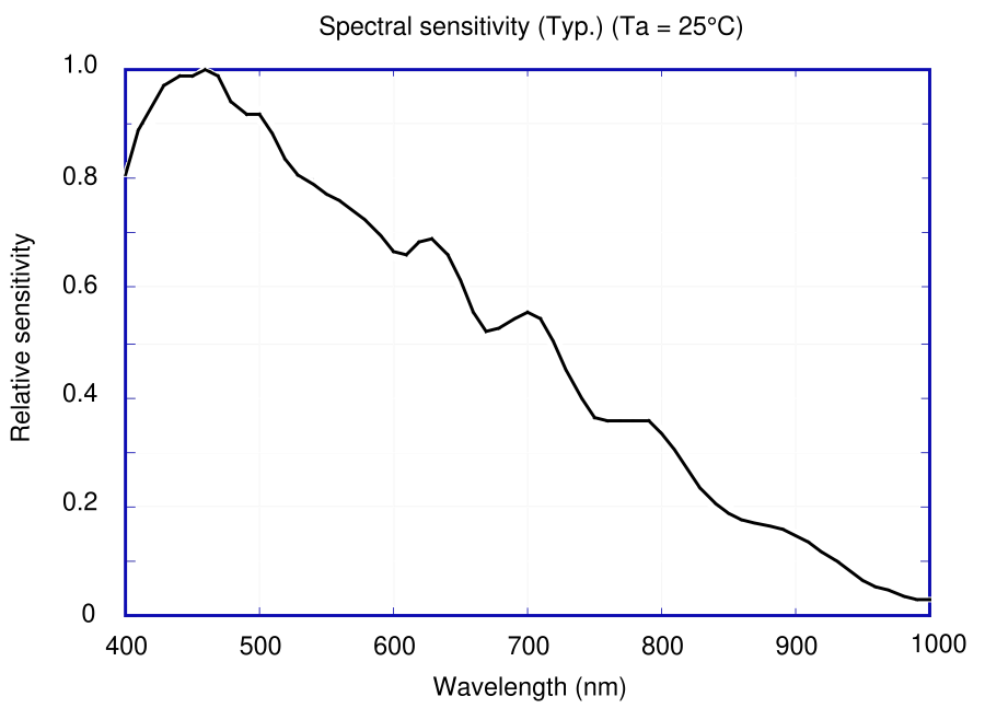
Failed conversion to floats

Nothing a bit of pdftocairo:

pdftocairo -r 2400 -png ILX511.pdf -f 8 -singlefile ilx-old

and gimp love couldn’t fix:

Gimped out the grid (mostly), recolored the axis, and even added teeny one-pixel red marks for the X1, X2, Y1, Y2 spots (500, 900, 0.1, 0.9)

After which it worked well:

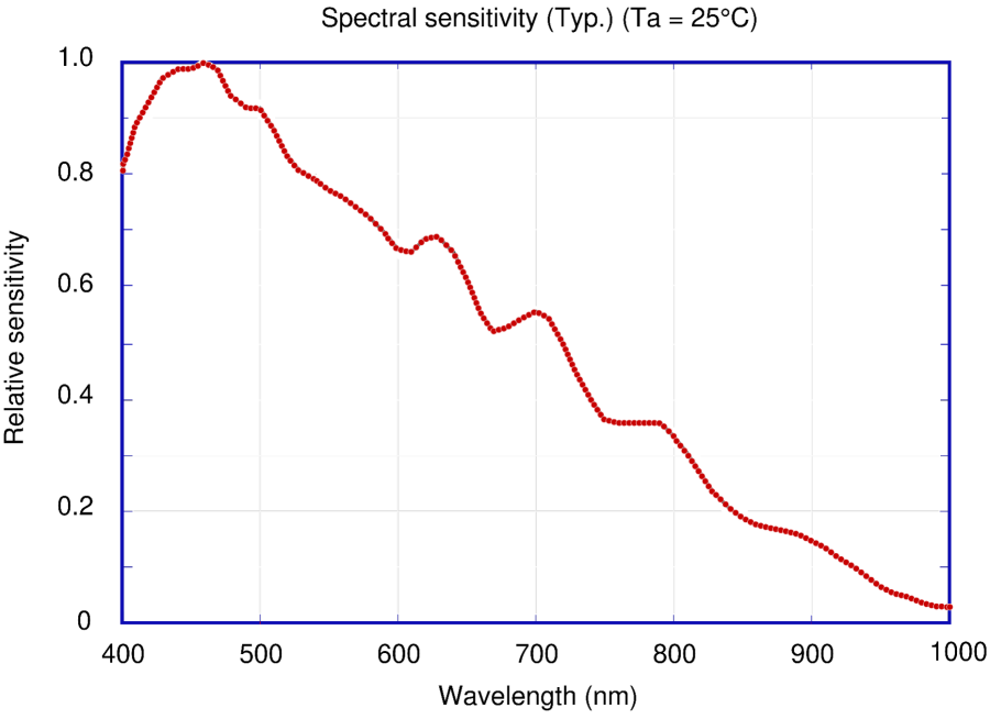Successful conversion to floats

Notice the much better resolution, because I went hog wild with 2400 dpi, resulting in 19834 x 28067 raw file trimmed down to 10288 x 7392.

That was a huge success, because saving the CSVs:

• SONY ILX511 spectral sensitivity
• SONY ILX511B spectral sensitivity

gave me the data needed (ILX511 sample):

>400.6758426916684, 0.8063234515811902
400.88530580103554, 0.8183199235748819
402.233450077073, 0.8257165255681422
...
994.3122834640396, 0.03020589465194501
998.2389145250553, 0.029199617702009517
1000.3496801423888, 0.02932951831005015

Now, with a bit of Mr. Python I could interpolate that to 1nm steps:

#!/usr/bin/env python3
"""Interpolates raw ilx511b sensitivities to 1nm steps"""

import csv
import json
import pprint
import sys

import numpy as np
from scipy.interpolate import interp1d
import matplotlib.pyplot as plt

wavelengths = []
intensities = []
#with open('sensitivity-fine.csv', newline='', encoding='utf-8') as csvfile:
with open('ilx-511-old.csv', newline='', encoding='utf-8') as csvfile:
    reader = csv.reader(csvfile)
    for ln in reader:
        if ln:
            wavelengths.append(float(ln[0].strip()))
            intensities.append(float(ln[1].strip()))

w_new = np.arange(340.0, 1025.0) # XXX: I know the orig data is 400..1000, sigh
i_new = interp1d(wavelengths, intensities, kind='linear', fill_value='extrapolate')(w_new)


if False:
    plt.plot(wavelengths, intensities, '-', label='Original Data', color='blue') 
    plt.plot(w_new, i_new, '-', label='Interpolated Data', color='red')

    plt.xlabel('X')
    plt.ylabel('Y')
    plt.title('Interpolation of Data')
    plt.legend()
    plt.grid(True)

    plt.show()

print(json.dumps(dict(zip(w_new.astype(int).astype(str), i_new)), indent=2))

and then with a bit of update to viz-scaled.rb from tobes-ui:

diff --git i/viz-scaled.rb w/viz-scaled.rb
index 7d31234..1020fe7 100644
--- i/viz-scaled.rb
+++ w/viz-scaled.rb
@@ -17,6 +17,7 @@ options = {
     max: true,
     rename: false,
     cmd: %w[python3 main.py -t overlay -d],
+    linearize_flame: false,
 }
 
 OptionParser.new do |opts|
@@ -38,6 +39,10 @@ OptionParser.new do |opts|
     opts.on('-c', '--command=CMD', "Tobes-ui command, default: #{options[:cmd]}") do |cmd|
         options[:command] = cmd
     end
+
+    opts.on('-l', '--[no-]linearize-flame', "Linearize FLAME-S data, default: #{options[:linearize_flame]}") do |lf|
+        options[:linearize_flame] = lf
+    end
 end.parse!
 
 if options[:wavelength] && options[:max]
@@ -53,6 +58,11 @@ Entries = Struct.new(:file, :wl, :max, :val_at_wl, :name, :data)
 
 entries = []
 
+ILX511=JSON.parse(File.read('ilx511.json')).map { |k,v| [k.to_i, v] }.to_h rescue nil
+def linearize_flame(wl, int)
+    int / ((ILX511 || {})[wl.to_i] || 1.0)
+end
+
 for file in ARGV
     begin
         name = nil
@@ -61,6 +71,9 @@ for file in ARGV
             file = $2
         end
         data = JSON.parse(File.read(file))
+        if options[:linearize_flame] && data['device'] =~ /^USB2000PLUS/
+            data['spd'] = data['spd'].map { |k, v| [k, linearize_flame(k, v)]}.to_h
+        end
         entries << Entries.new(
             name || file,
             Range.new(*data["wavelength_range"]),

I could plot (ruby viz-scaled.rb -l -n -w 550 examples/overcast-*json) the result.

Did that help?

Well, no:

After linearization by ILX511 curve (limited to 400..1000 due to artifacts)

and no:

After linearization by ILX511B curve

I mean… it’s better, but not nearly enough.

In other words, some other approach is needed.

Closing words

My next try is going to be calibrating against a few blackbodies (halogen incandescent bulbs) by curve fitting the response to the ideal curve and deriving the coefficients that way.

Hopefully that gets me closer to where I want to go⁷.

Stay tuned.

But in any case, I have a newfound respect for spectrography. Shit ain’t as easy as it seems, yo. Is this G….e?